


INTRODUCTION
Sequential analysis is a statistical method in which the final number of patients analyzed is not predetermined, but sampling or enrollment of patients is decided by a predetermined stopping rule such as satisfying a statistical significance. Accordingly, the investigators may draw a conclusion earlier than that with the traditional statistical methods, reducing time, cost, effort, and resources.
The concept and method of sequential analysis were introduced and described as expeditious industrial quality control methods during World War II by Abraham Wald [1]. This concept was used to prove the desired or undesired intervention effects by analyzing data from ongoing trials. After World War II, Peter Armitage introduced a sequential analysis method to medical research and suggested applying a strict significance level to stop a trial before a predetermined number of patients was reached [2].
A systematic review is a research method that attempts to collect all empirical evidence according to predefined inclusion and exclusion criteria to answer specific and focused questions [3]. It uses clear, transparent, and explicit methods to minimize bias, providing more reliable information [4]. Meta-analysis is a statistical analytic method that integrates and summarizes the results from individual studies or examines the sources of heterogeneity among studies [5].
Systematic review and meta-analysis rank highest in evidence hierarchy and provides evidence for clinical practice, healthcare, and policy development. Its use and application in clinical practice have increased [6,7]; however, they are not free from errors and biases [8]. Many systematic reviews and meta-analyses have included too few studies and patients to obtain sufficient statistical power, leading to spurious positive results [9]. Some positive findings from the meta-analysis may be caused by a random error (by chance) rather than the true effects of the intervention. Therefore, results from systematic reviews and meta-analyses may often increase the likelihood of overestimation (Type I errors) or underestimation (Type II errors) [10,11]. Furthermore, because meta-analysis can be updated when there is a new clinical trial, the inflation of Type I and II errors from multiple and sequential testing is of major concern [12].
Trial sequential analysis (TSA) has been developed to resolve these problems. Conceptually, TSA adopts sequential analysis methods for systematic reviews and meta-analyses. However, TSA is different from sequential analysis in a single trial in that the enrolled unit is not a patient but a study. Sequential analysis is performed at predetermined, regular intervals, although the number of enrolled patients did not reach predetermined number of patients. However, in TSA, the trials were included in chronological order, and analysis was performed repetitively and cumulatively after new trials were conducted. TSA also provided an adjusted significance level for controlling Type I and II errors. Therefore, the adaptation of TSA when performing and presenting a meta-analysis has been increasing recently [13,14].
This article aims to describe the history, background, principles, and assumptions behind the use and interpretation of TSA.
BACKGROUND AND PRINCIPLE OF TRIAL SEQUENTIAL ANALYSIS
Required information size
Meta-analysis is a statistical method used to synthesize a pooled estimate by combining the estimates of two or more individual studies. As the number of events or patients increase, the power and precision of the intervention effect estimate also increases. Thus, a more reliable estimate can be obtained from meta-analysis than a single randomized controlled trial (RCT) [4].
A single RCT performs sample size calculation or power analysis to ensure that the study provides reliable statistical inference and targeted power. Similar to sample size calculation or power analysis in a single RCT, the required information size (RIS) or optimum information size was proposed and used in the meta-analysis.
The RIS in meta-analysis is defined as the number of events or patients from the included studies necessary to accept or reject the statistical hypothesis [15].
The sample size calculation performed in a single RCT is based on the effect size, significance level, and power [16]. In a single RCT setting, predetermined homogenous patients, intervention, and methodology are used. However, in a meta-analysis setting, a wide range of patients, regimens of intervention, different experimental environments, and quality of methodology may be applied in each study. Heterogeneity may arise across the included studies, which increases the sample size needed to accept or reject the statistical hypothesis. Therefore, the RIS in meta-analysis should be adjusted considering the heterogeneity between included studies and should be at least as large as the sample size in a homogenous single RCT [15].
As in a single RCT, assumptions to calculate RIS should be predefined before the systematic review and meta-analysis. A single RCT with too few patients is thought to have low precision and power. Similarly, results from meta-analyses with too few studies and patients are assumed to have an increased likelihood of overestimation or underestimation due to lack of precision and power in the intervention effect [10,17]. Therefore, the use of appropriate RIS is important to increase the quality of meta-analysis.
The TSA program (Copenhagen Trial Unit, Centre for Clinical Intervention Research, Denmark) provides a simple and useful way to calculate the RIS. The TSA program uses the heterogeneity-adjustment factor (AF) to adjust for heterogeneity among the included trials. AF is calculated as the total variance in a random-effects model divided by the total variance in a fixed-effect model as follows:
AF: heterogeneity-adjustment factor
VR: total variance in a random-effects model
VF: total variance in a fixed-effect model
Because the total variance in a random-effects model is greater than or equal to the total variance in a fixed-effect model (VR ≥VF), AF is always greater than or equal to 1.
Finally, the RIS adjusted for heterogeneity between trials (random) is calculated by multiplying the non-adjusted RIS (fixed) with AF.
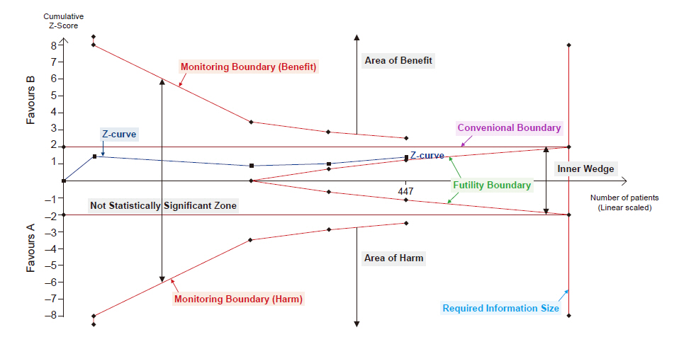
In the TSA program, RIS is automatically calculated by defining the statistical hypotheses, namely information size, Type I error, power, relative risk reduction, incidence in the intervention and control arms, and heterogeneity correction in the Alpha-spending boundaries setting window is activated in TSA tab and displayed in the TSA diagram (Fig. 1). This will be discussed later in TSA tab section.
Alpha spending functions and monitoring boundaries
Type I error, or false positive, is the error of rejecting a null hypothesis when it is true, and Type II error, or false negative, is the error of accepting a null hypothesis when the alternative hypothesis is true. Intuitively, Type I error occurs when a statistical difference is observed, although there is no statistically significant difference in truth, and Type II error occurs when a statistical difference is not observed, even when there is a statistical difference in truth (Table 1).
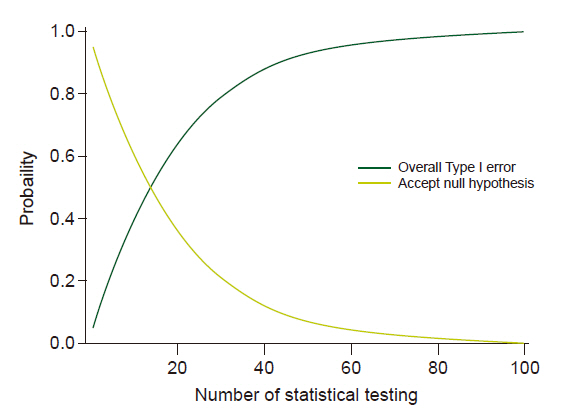
Multiple comparisons and multiple testing problems occur when data is sampled repeatedly from the same data set, data is analyzed simultaneously or multiple times, or data is analyzed sequentially by observing more results. Multiple comparisons inflate the possibility of a Type I error (α). For example, if statistical analysis is performed at a significance level of 5% and the null hypothesis for statistical analysis is true, there is a 5% chance for a Type I error. However, if statistical analyses were performed 100 times for the same situation, the expected number of Type I errors would be 5, and the probability of occurrence of at least one Type I error would be 99.45% (Fig. 2). Therefore, it is very important to adjust the α level so that the overall Type I error remains within the desired level.
An interim analysis before the completion of data collection may also cause inflation of Type I error in the absence of appropriate adjustment. During clinical trials, the researchers may stop the trial early via predefined strategies, such as observation of clearly beneficial or harmful effects in the test group compared to the control group or if interim analysis shows futile results. Trials with interim analysis inevitably have plans for two or more statistical analyses. Therefore, when planning an interim analysis, a plan for appropriate adjustment of the α-level considering inflation of Type I error from multiple comparisons should be considered.
Several statistical methods have been proposed for adjusting the α-level. These methods generally require a significance level for each comparison that is strict and conservative in adjusting the inflation of Type I error.
Of these, the method proposed by Bonferroni is the simplest and is most frequently used to adjust the statistical significance threshold. The Bonferroni correction method is conducted by dividing the desired overall α-level by the number of analyses (hypothesis). However, it is based on the assumption that the data are independent and cannot be used for a dependent dataset, such as interim analysis or TSA. It has also been criticized for its conservativeness [18].
Group sequential analysis, proposed by Armitage and Pocock, is another method to adjust the significant threshold. Similar to the Bonferroni correction method, the overall risk of Type I error is restricted within the desired overall α-level by dividing the desired overall α-level by the number of analyses performed. However, this method is used for data- dependent analyses such as interim analysis. In the method proposed by Richard Peto, the Type I error from four interim analyses is set at 0.001, and the Type I error in the final analysis at 0.05 [19]. However, these methods have a limitation in that the number of analyzed data should be predefined, and the analyzing interval should be equal.
In a single RCT, an interim analysis is determined and planned before the start; thus, it is possible to know the number of analyses, including interim and final analysis and analysis intervals. However, meta-analyses are generally updated when new clinical trials are performed. Furthermore, the intervals between trials are arbitrary and irregular, and the number of included patients is unpredictable [12]. For these reasons, the methods proposed by Bonferroni, Armitage and Pocock or Peto are not applicable for meta-analysis. For flexibility in analysis, in terms of interval and patients included, O’Brien and Fleming [20] proposed a method for interim analysis in a single RCT, and it was later developed further by Lan and DeMets [21-23]. This method does not impose restrictions, such as the interval between analysis and the number of patients, but depends on the parameter chosen for the spending function.
The TSA program provided statistical monitoring boundaries that show a sensible threshold for statistical significance (alpha spending functions) based on methods developed by Lan and DeMets [21-23]. In the TSA program, alpha spending functions are automatically calculated, and statistical monitoring boundaries are displayed in the TSA diagram (Fig. 1). The monitoring boundaries presented in TSA are dependent on the RIS fraction, which was included in the meta-analysis [15]. The lower the number of patients reached compared with RIS, the higher the intervention uncertainty. In contrast, when the closer the number of patients that reach the RIS, the uncertainty decreases. As uncertainty increases, the statistical significance level decreases, and the significance interval widens. Thus, when the fraction of RIS is small, the interval between the monitoring boundaries becomes wider.
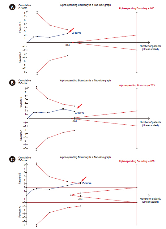
Fig. 3A shows that the last point in the z-curve is outside of the conventional test boundary but within the monitoring boundaries. Therefore, we can conclude that there is a statistical difference in the conventional meta-analysis, but we cannot conclude a statistical difference in TSA. When adding a new trial and updated TSA (with adding 79 patients, number of patients included in the TSA increased from 244 [Fig. 3A] to 323 [Fig. 3B or C]), the last point in the z-curve may remain within the monitoring boundaries (‘Not Statistically Significant Zone’) (Fig. 3B) or outside the monitoring boundaries to reach ‘Area of Benefit’ (Fig. 3C). Thus, the pooled estimates in TSA may become statistically nonsignificant (Fig. 3B) or significant (Fig. 3C) after the addition of the new trial. In that case, we either conclude that intervention has an effect (Fig. 3C) or further studies are needed as a conclusion could not be derived (Fig. 3B). The construction of the monitoring boundaries in the TSA program will be discussed in TSA tab section.
Beta spending functions and Futility boundary
If the result of the meta-analysis was negative and the appropriate RIS was reached, we can easily conclude no effect of the intervention. However, if the result of the meta-analysis was negative and appropriate RIS was not reached, two possibilities exist: no effect of the intervention or lack of power.
If we can assume that the intervention is unlikely to have an anticipated effect before reaching RIS, we can prevent spending time, money, effort, and limited resources on unnecessary further trials. Therefore, TSA provides ‘Futility boundaries’ or ‘inner wedge’, which is the adjusted threshold for non-superiority and non-inferiority tests (Fig. 1). It was originally developed for sequential analyses. If the pooled effect of the estimate lies within the futility boundaries, we can conclude that the intervention is unlikely to have an anticipated effect. If the pooled effect of the estimate lies within the monitoring boundaries (statistical significance), but outside the futility boundaries, we cannot conclude whether the negative effect arises from a lack of power or due to the unlikeliness of the intervention to have an anticipated effect.
The possibility of inflating Type II errors also exists for multiple and sequential analyses in meta-analysis. Similar to the alpha spending function, the methods proposed by Lan and DeMets [21-23] can be extended to control Type II errors. In the TSA program, futility boundaries are provided using the methodology proposed by Lan and DeMets and reflect the uncertainty of obtaining a chance negative finding in relation to the strength of the available evidence (e.g., the accumulated number of patients).
Fig. 4A shows that the last point in the z-curve stays outside the futility borders but within the conventional test boundaries. In this case, we cannot conclude whether the intervention is unlikely to have an anticipated effect. When adding a new trial and updating the TSA (with adding 101 patients, number of patients included in the TSA increased from 346 [Fig. 4A] to 447 [Fig. 4B or C]), the last point in the z-curve is within the futility borders (‘inner wedge’) (Fig. 4B) or stays out of futility borders and within monitoring boundaries (Fig. 4C). In these cases, we can conclude that the intervention has no effect (Fig. 4B) or cannot conclude whether the negative effects arise from a lack of power or whether the intervention is unlikely to have an anticipated effect.
The cumulative test statistic (Z-curve)
The TSA program uses the Z-statistic or the Z-value, which is calculated by dividing the log of the pooled intervention effect by its standard error (Fig. 1). Z-statistics are assumed to follow a standard normal distribution, with a mean of 0 and a standard deviation of 1. The larger the absolute value of the Z-value, the larger the probabilities that the two interventions are different, and these differences cannot be explained by chance. As P value is the probability of finding the difference between the observed difference or if the null hypothesis is true, P and Z-values are interchangeable and can be inferred from Z-value (for example, a two-sided P value of 5% represents Z-value of 1.96). Whenever a meta-analysis is updated, the TSA program calculates the corresponding Z-value and then provides a Z-curve that plots the series of consecutive cumulative Z-statistics.
The law of the iterated logarithm
Another approach to adjust the issues of repeated significance testing is to penalize the Z-values by the strength of the available evidence and number of statistical tests. The TSA program uses the law of iterated logarithms for this purpose.
The law of the iterated logarithms states that if data are normally distributed, data divided by the logarithm of the logarithm of the number of observations will exist between - 2 2
The adjusted (penalized) Z-value, Zj*, is calculated as follows:
Zj: the conventional Z-value at the j-th significance test
Ij: the cumulative statistical information at the j-th significance test
λ: constant control for maximum Type I error
λ is constant to control for Type I errors, and various values have been suggested for various situations. For continuous data meta-analysis, λ = 2 is known to control Type I error at α = 5% for a two-sided test [23]. However, dichotomous data and appropriate λ values are suggested differently according to the type of measure and Type I error [24] (Table 2).
Effect measure
For dichotomous data, the TSA program uses relative risk (RR), risk difference (RD), odds ratio (OR), and Peto’s odds ratio as the effect measure for meta-analysis. When events are rare, Peto’s odds ratio is the preferred effect measure for meta-analysis.
Table 3 presents the 2 × 2 contingency tables for dichotomous data.
In Table 3, the risk of an event in the experimental group (pT) is a a + b c c + d R R = p T p C = a a + b c c + d = ( c + d ) × a ( a + b ) × c
RD, which is conceptually similar to the relative risk reduction used in TSA, is defined as R D = p T - p C = a a + b - c c + d
Odds is defined as the P r o b a b i l i t y o f a n e v e n t P r o b a b i l i t y o f o f a n n o n - e v e n t a a + b p T 1 - p T = a a + b 1 - a a + b = a a + b ( a + b ) - a a + b = a a = b b a + b = a b c d
The Peto odds ratio is defined as ORPeto=exp((eA-E(eA))/v, where eA is the expected number of events in intervention group A, and ν is the hypergeometric variance of eA.
For continuous data, the TSA program uses mean difference as the effect measure to perform a meta-analysis. However, the TSA program does not support meta-analysis using the standardized mean difference.
Model
The TSA program provides four models to integrate effective sizes: 1) fixed effect model, and random effect models using the 2) DerSimonian-Laird (DL) method, 3) Sidik-Jonkman (SJ) method, and 4) Biggerstaff-Tweedie (BT) method.
The fixed effect model is applied based on the assumption that the treatment effect is the same, and the variance between studies is only due to random errors. Thus, the fixed effect model can be used when the studies are considered homogeneous; namely, the same design, intervention, and methodology are used in the combined studies, and the number of included studies is very small. In contrast, the random effect model assumes that the combined studies are heterogeneous, and the variance between studies is due to random error and between-study variability [5]. The random effect model may be used when the design, intervention, and methodology used in the included studies are different. TSA program provides three different methods to integrate the effect estimate. The DL method is the most commonly used and simplest random effect model and is the only option for Review Manager software (Nordic Cochrane Centre, Denmark). However, DL method tends to underestimate the between-trial variance. This can be overcome by the SJ method that applies a noniterative estimate of the variance based on re-parametrization [25]. SJ method reduces the risk of Type I error compared with DL method. In a meta-analysis with moderate or substantial heterogeneity, the false positive rate based on the SJ method was estimated to be close to the desired level (conventionally 5%), but the false positive rate based on the DL method increased from 8% to 20% [25]. However, the SJ method has the risk of creating too wide a confidence interval by overestimating the between-trial variance, especially in meta-analyses with mild heterogeneity. BT method incorporates the uncertainty of estimating the between-trial variance and minimizes the effect of the bias via appropriate weighting in large trials, especially when the size of the trials varied and small trials were biased [26].
The choice of model should be based on a comprehensive understanding of the strength and weaknesses of these models and should involve a sensitivity analysis for each model.
Methods for handling zero-event trials
The TSA program provides three methods for handling zero-event trials. Some studies with dichotomous data have zero events in the intervention or control groups. In this case, the estimate measures (RR and OR) of the intervention effect are not meaningful [27]. To address this problem, continuity correction, where we add some constant to the number of events and nonevents in the compared groups, can be the statistical solution.
In constant continuity correction, a constant is added to the number of events and nonevents in all groups. This method is simple and the most commonly used. The continuity correction factor commonly used in Review Manager software is 0.5. This method yields some problems, such as inaccurate estimation of intervention when the randomization ratio to groups are not equal or too narrow confidence interval is induced [27].
In reciprocal of opposite intervention group continuity correction, also known as ‘treatment arm’ continuity correction, the number of events divided by total number of patients in each intervention group is added to the reciprocal intervention group.
The intervention effect is estimated toward ‘the null effect’ (i.e., towards 1 for RR or OR and 0 for RD) in both correction methods. In contrast, empirical continuity correction is known to estimate the effect measure for meta-analysis results [27].
USING THE TSA PROGRAM
The TSA shows the menu bars at the start of the program: File, Batch, and Review Manager. Under these menu bars, another row, namely Meta-analysis, Trials, TSA, Graphs, and Diversity, are located. We can start a new meta-analysis project by clicking the New Meta-analysis sub-menu under the File menu bar. Then, a New Meta-analysis window will be created with a drop-box named Data Type, blanks named Name, Label for Group 1, Label for Group 2, and Comments, and check-box named Outcome type. By entering or selecting appropriate information in the New Meta-analysis window, we can create a new meta-analysis. Here, we can choose dichotomous or continuous Data Type drop-box and negative or positive in the Outcome type check-box.
Meta-analysis tab
When a new meta-analysis is created, the Meta-analysis tab will be activated, and the name of the new meta-analysis will appear in the upper middle part of the window, the Set Effect Measure and Model, Set Zero Event Handling, and Set Confidence Intervals area will appear on the left side of the window, and the Meta-analysis Summary area will appear in the middle of the window.
Within the Set Effect Measure and Model area, there are two drop-boxes named the Effect Measure and Model. In the Effect Measure drop-box, we can choose among Relative Risk, Risk Difference, Odds Ratio, and Peto Odds Ratio when the data type is dichotomous, and Mean Difference when the data type is continuous. A detailed description of the effect measure is provided in Effect measure section. We can choose Fixed Effect Model or Random Effect Models DL, SJ, and BT in the Model drop-box. A detailed description of the model is provided in Model section.
When the data type is dichotomous, the Set Zero Event Handling area is activated. Within the Set Zero Event Handling area, there are two drop-boxes named Method and Value and a check-box named Include trials with no events. We can choose among Constant, Reciprocal, Empirical options in the Method drop-box, and 1.0, 0.5, 0.1, and 0.01 in the Value drop-box. We can also choose whether to apply continuity correction or not using Include trials with no event check-box. A detailed description of the handling zero-event data is provided in Methods for handling zero-event trials section. Within the Set Confidence Intervals area, we can choose between Conventional (coverage) (with confidence intervals of 95%, 99%, and 99.5%) or α-Spending adjusted CI check-box. For the adjusted significance test boundaries (see detail in TSA tab section), α-Spending adjusted CIs functions are available. When α-Spending adjusted CI is checked, the select tab is activated. Simultaneously, the Alpha-spending Boundary window will be activated, and we can choose from among the available options.
Trials tab
TSA programs provide the option to import meta-analysis data saved in the Review Manager v.5 file (*.rm5) through RM5 Converter, shown in the menu bar of the TSA program. We can also add, edit, and delete trials using the Trials tab.
When clicking on the Trials tab, Add Dichotomous Trial or Add Continuous Trial according to the type of data, Edit/Delete Trial, and Ignore Trials area will appear on the left side of the window.
In both dichotomous and continuous trials, we can input the study name (Study) and publication year (Year), comment on each trial (Comment) in the blank space, and select whether the study has low risk bias (Low Bias Risk check box). Further, we can input the number of events (Event) and total number of patients (Total) for each group in Add Dichotomous Trial and mean (Mean Response), standard deviation (Standard Deviation), and total number of patients (Group Size) for each group in Add Continuous Trial.
The added trial will appear on the right side of the window, containing the Study, Bias Risk, Ignore, and Data columns. The Study column contains the year (left and within parenthesis) and name of trial (right). The Bias Risk column contains the bias risk of corresponding trials (low [in green] or high [in red]), and the Data column contains data for each trial. We can also ignore the trials using the check box in the Ignore column. By clicking the “Edit Selected” or “Delete Selected” button in Edit/Delete Trial, we can edit or delete the trial, respectively. We can also select or ignore the low and high bias risk trials using the Low Bias Risk trials, Hish Bias Risk trials, All or Ignore buttons in Ignore Trials area.
TSA tab
When the TSA tab is activated, the Add area appears on the left upper side of the window. There are three buttons within the Add area: Conventional Test Boundary, Alpha-spending Boundaries, and Law of the Iterated Logarithm, where we can apply the type of significance test. Clicking on the Conventional Test Boundary button activates the Add Conventional Test window, in which the name of test (Name) and Type Ⅰ error (Type Ⅰ error) can be specified and the Boundary type (one-sided upper, one-sided lower, and two-sided) can be selected. The TSA program provides a linear conventional test boundary according to the boundary type and Type Ⅰ error applied in the TSA graph.
The alpha-spending Boundaries button activates the Add Dichotomous Alpha-spending Boundary or Add Dichotomous Alpha-spending Boundary window according to the data type. In both windows, there are Boundary Identifier, Hypothesis Testing, and RIS areas. The two windows differ in terms of the RIS area.
In the Boundary Identifier area, we can name the test applied (Name). In the Hypothesis Testing area, there are Boundary Type and Information Axis check-boxes and α-spending Function drop-boxes. The Boundary Type enables choosing the type of boundary (One-sided Upper, Ones-sided Lower, and Two-sided), and Information Axis allows choosing the type of information as the number of patients included (Sample Size), number of events (Event Size), or Statistical Information. We can also set the Type I error value and choose whether to apply the inner wedge using the Apply Inner Wedge check-box. The Apply Inner Wedge enables testing for futility by choosing the level of Type II error (Power) and β-spending Function. For both the α- and β-spending Function, only the O’Brien-Fleming function is available in the TSA program.
In the RIS area for continuous data, we can specify the Type Ⅰ error and Power and choose Information Size (User Defined and Estimate), Mean Difference (User Defined, Empirical, and Low Bias), Variance (User Defined, Empirical, and Low Bias), and Heterogeneity Correction (User Defined and Model Variance Based). In the RIS area for dichotomous data, we can specify the Type I error and Power and choose Information Size (User Defined and Estimate), Relative Risk Reduction (User Defined and Estimate), Incidence in Intervention arm (User defined), and Heterogeneity Correction (User Defined and Model Variance Based). The RIS area can be left blank or available options for the RIS calculation can be selected. To estimate RIS, we can input any arbitrary number obtained under the User defined option. Then, the RIS can be automatically generated according to the type of information gathered.
For continuous data, Mean Difference and Variance have three options: User Defined, Empirical, and Low Bias. When selecting User Defined, we use an arbitrary number. However, we can use pooled estimates of intervention from all studies (under the option Empirical) and low-risk bias trials (under the option Low Bias). For dichotomous data, Relative Risk Reduction and Incidence in Intervention arm have the option User Defined and Low Bias Based. The definitions for these options are similar to those for continuous data.
The heterogeneity correction tab adjusts the ratio between the variance in the random effect model and fixed model (Model Variance Based) and predicts the heterogeneity based on prior studies (User defined) as the ratio of trial variations to the total variance.
After making Alpha-spending Boundaries, we can add the timing of interim looks, namely when the meta-analysis was performed, by selecting the trials in the interim analyses area on the right side of the window.
The Law of the Iterated Logarithm button activates the Add Law of Iterated Logarithm window to perform the significance test by penalizing the Z-curve. In this window, there are Boundary Identifier, Boundary Settings, and Penalty areas. In the Boundary Identifier area, we can name the test applied. Boundary Settings include Boundary Type (One-sided Upper, Ones-sided Lower, and Two-sided) and Type I error rate. For λ we can use the numbers in Table 2. Detailed explanations for λ are described in the law of the iterated logarithm section. The Edit area, under the Add area, contains the Edit Selected and Delete Selected buttons to edit or delete the significance test, respectively.
In the lower left corner are the Templates area, with the options for saving the constructed significance tests using Add-to-Templates button or loading the saved significance tests using the Manage templates button. The Information Axis (sample size, event size, and statistical information) checkbox is located on the left side of the window.
To perform the analysis using TSA program, we use the Perform calculations button in the Calculations area.
Graphs tab
When the Graphs tab is checked, the Tests and Boundaries Layout area, Set Graph Layout area, Print Current Graph button, and Generate TSA report button appear on the left side of the window.
The Tests and Boundaries Layout allows changing the color, line type, line width, icon at each trial, icon size, font size, and font size in the graph. It also provides the option to show and hide the presented graph.
The Set Graph Layout area has Trial Distance drop-boxes and Layout setting buttons. The Trial Distance drop-box allows setting the distance between boundaries and between the Z-values according to the amount of information (Scaled), or an equal distance is set between trials on the information axis (Equal).
The Layout setting button activates the Graph Layout Settings window to adjust the line width and font size of the x- and y-axis, font type, and font size.
In the middle of the window and above the TSA graph, there are two tabs: Adjusted Boundaries and Penalised Tests representing adjusted significance tests based on α-spending functions and law of the iterated logarithm penalties, respectively. The former represents the adjusted thresholds for the Z-curve, and the latter represents the adjusted test statistics in relation to the single-test significance test threshold.
Diversity tab
The TSA program provides diversity estimates for the random effect models using the DL method (Random DL), SJ method (Random SJ), and BT method (Random BT).
When diversity Tab is activated, each trial and its weight percentage for each model, fixed effect model, random DL, random SJ, and random BT models are displayed in the upper part of the window.
In the left lower corner, various diversity types, I2 (estimate of inconsistency) and 1/(1-I2) (heterogeneity correction for estimating inconsistency), D2 (estimating diversity), and 1/(1-D2) (heterogeneity correction for estimating diversity), and Tau (of between-trial variance) for the three random effect models are displayed.
Criticism for TSA
The use of TSA has increased recently [4,28] because it can reduce the probability of false positives and false negatives owing to random errors and provide early detection of the acceptance or rejection of the intervention effect. However, TSA is criticized owing to some concerns [28,29]. Firstly, TSA is a complex statistical tool that is not easy to perform and can be misused as clinicians are not familiar with it. The Cochrane Scientific Committee Expert Panel is also against the routine use of TSA. Secondly, TSA is retrospective and observational, as in conventional meta-analysis, and it thus has the risk of data-driven hypotheses. Therefore, to avoid this risk, the protocol for systematic review and TSA, including hypothesis, anticipated effect of intervention, proportion of outcome in the control group, heterogeneity, and meta-analytic model, should undergo either peer-review or be made publicly available on open-access platforms. Thirdly, we cannot adopt the results of TSA to finalized studies. In a single RCT, the interim analysis results, showing the benefits, harm, or no intervention effects, affect the decision to continue or stop the trial. However, we cannot control those studies that have already been performed. Finally, TSA provides results that are too conservative in applying desired interventions in the clinical field.
CONCLUSION
Systematic review and meta-analysis rank highest in the evidence hierarchy and has been widely used recently. However, these involve too few studies and participants, resulting in spurious results. The adjusted significance level controlling for Type I and II errors with TSA, provides information on the precision and uncertainty of the meta-analysis results. TSA also provides monitoring boundaries or futility boundaries; therefore, providing information on whether ongoing trials are necessary, thus preventing unnecessary trials. However, as the principle behind TSA is complex, we are prone to misuse it.
This article provides the basic principles, assumptions, and limitations to understand and interpret TSA. When TSA is properly performed and interpreted, it can be a powerful tool to clinicians, patients, and policymakers providing results that are only achieved by large-scale RCTs.